Using Evolutionary Computation to Explain Network Growth

Our article titled “Symbolic regression of generative network models” has finally been published. I am really happy with the final result and the fact that it is open access.

Explaining network growth is a challenge that appears in a surprising number of disciplines. For example, neuroscientists are interested in understanding how brains develop, and sociologists in how social networks acquire a certain topology.

Finding plausible explanations is not trivial. Real networks tend to be large and complex. Reverse-engineering the growth process from a snapshot of a network is a problem that easily defeats human intuition.

So we developed a method to look for such explanations automatically. We employ evolutionary computation, a machine learning technique inspired by natural selection. Network growth processes (a.k.a. network generators) are represented by simple computer programs. In other words, using only the snapshot of a given network, our method automatically discovers simple laws plausibly governing its evolution. For instance, from an empirical political blog network (see below) we find an equation as simple as exp(4−2d).

This suggests that a generative process giving exponential priority to closer nodes is able to successfully reconstruct many key features of the original network.

The evolutionary process evaluates the quality of generators by creating synthetic networks according to the growth process they define and then comparing these synthetic networks to the target, real network. The comparison is done using a set of well-known metrics that target both macro and micro-level features of the networks.

The best way to understand the method is, of course, to read the paper .

We are also releasing an open-source software tool called Synthetic that any researcher can apply to their own networks. If you are interested, don’t hesitate to contact us. We would love to hear from any attempts (successful or not) at using Synthetic outside of our lab.

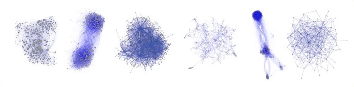
To illustrate what can be achieved, I leave you with seven generators we discovered. They cover very different types of networks, including a simple brain, protein interactions and social networks. The following table describes the variables used in the expressions:

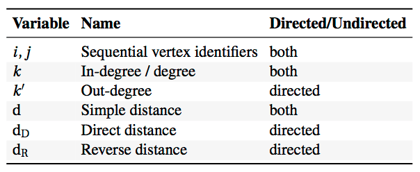
The expressions that define the generators use these variables to assign weights to the pairs of unconnected nodes in the network. The higher the weight, the more likely it is that the generator will establish a connection between the nodes.

A simple example: consider a “rich get richer” phenomena. The more incoming connection a node has, the more likely it is to receive more connections. Such a generator could be defined as:

$$w(i,j)=k(j)$$

The following examples are roughly ordered by increasing complexity of the generator.

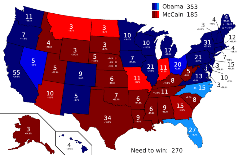
Political Blogs

Citation network of political blogs during the 2004 American presidential elections

$$w(i, j) = exp(4 – 2d)$$

The political blogs generator takes a single variable: $d$. Unlike with $d_D$, the case where d=1 can happen, as this distance may be caused by an arc with the opposite direction of the one being proposed. This generator behaviour can be simply described, as shown in the following figure:

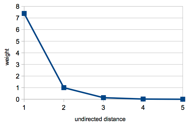
Reciprocity is strongly encouraged, given the high weight given to arcs with $d=1$.

In fact, this situation necessarily corresponds to a reciprocal arc (linking to a blog that linked to you), because arcs that already exist are not allowed in the sample. Then, weight decreases as undirected distance increases, but never to 0. This distribution of weights according to undirected distances is sufficient to generate the two communities in the network — links between blogs that have a low undirected distance are more probable, but links to more distant blogs are also possible. This leads to the low density of links between the two communities. Surprisingly, it is possible to propose a plausible generator that leads to the two communities without resorting to a priori diversity (e.g Democrats vs. Republicans), that could be expressed with sequential identifiers or the affinity function. It can be speculated that this matches the way in which political ideology propagates in society.

Word Adjacencies

Network of word adjacencies in the novel David Copperfield by Charles Dickens

$$w(i, j) = k(i) – d$$

This network represents the adjacencies of common adjectives and nouns in the novel “David Copperfield” by Charles Dickens.

The generator configures a simple combination of preferential attachment with a preference for connecting to close vertices. An increase in the degree of a node also increases its reach, as the distance term can be higher with making the weight negative, and thus null.

Facebook

Neighbourhood of a single Facebook user

$$w(i, j) = \psi(3, i \cdot k(i), k(i))$$

The facebook generator combines preferential attachment with affinity in a simple fashion. The constant value for the number of groups suggests pre-existing social circles.

• affinity: $i \cdot k(i)$
• no affinity: $k(i)$

The role of the factor $i$ in case of affinity appears to be two-fold: increase the propensity for connections inside pre-existing social circles (for the most cases $i > 1$) and capture an external preference for certain connections within such groups over others. This matches the intuition that popularity in the real world is expressed in the facebook social graph.

Connections between groups follow a pure preferential attachment regime, matching the intuition that more popular individuals are more likely to act as bridges between communities.

C. Elegans

Brain of a C. Elegans roundworm

$$w(i, j) = log(d_D)d_D – 7 – min(j + 0.52, 0.77)$$

The C.elegans generator uses two variables: $d_D$ and $j$. Given the term where $j$ appears, $min(j + 0.52, 0.77)$, a distinction is only made between $j = 0$ and $j > 0$. For the first case, the term takes the value $0.52$, for the second the value $0.77$. The first term uses the $d_D$ variable, which takes integer values in ${0, …, 5}$. Only values equal to or greater than $2$ are relevant, given that $d_D = 0$ configures a self-link, while $d_D = 1$ indicates an already existing arc. Both these situations are prohibited in the configuration we use.

As negative values are considered null weights, we can reduce the generator to $3$ possible situations, shown in the following table:

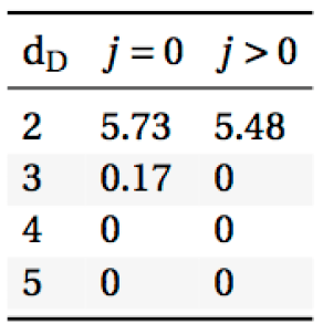
Here we can see that the rule is indeed very simple: the generator promotes the creation of A→B arcs where an A→C→B arc already exists ($d_D = 2$). For the special case of an arc where the target has the sequential identifier $0$, $d_D = 3$ is also allowed, albeit with a much lower probability. For $d_D = 2$, connection to this special node are also slightly preferred.

Sequential identifiers are abstractions meant to capture some a priori heterogeneity in the vertex set, so the meaning of the special node 0 can only be speculated on. It might represent a certain spatial constraint for a neuron or a different behaviour of the neuron through some mechanism. Such interpretations are beyond the scope of the work and better left to researchers with the adequate domain knowledge.

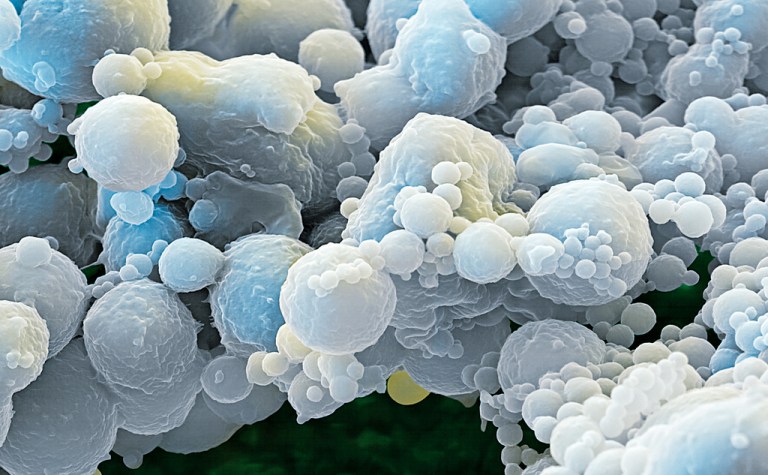
Proteins

A network of protein interactions in Homo Sapiens

$$w(i,j)=⎧⎨⎩log(i),if k(j)={0,if k(i) < 4k(i),otherwise−1,otherwise$$

The protein interactions generator only assigns a non-null weight in two cases: if the target is not yet connected and the origin has a low degree ($k(i) < 4$), or if the degree of the origin and target are the same. Non-null weights are always $log(i)$, indicating an a priori logarithmically distributed propensity for interaction.

This generative process seems to indicate a strong preference for assortativity on degree, establishing edges between proteins that interact with a similar number of other proteins.

Software Collaborations

Collaboration network of authors from the CPAN Perl module repository

$$w(i,j)=\psi(k’(i)d,k’(j),0.7k(j))⋅min(k(j),9)$$

The software collaborations network represents software authors from the CPAN Perl language repository. An arc means then an author uses a software module from another author.

Here we can see that the affinity operator is used. The first parameter of the operator represents the number of groups that the vertex set is divided into, so the higher this value, the less likely affinity between to arbitrary vertices becomes. The number of groups is rounded to the closest integer.

As the number of groups is determined by k′(i)d, an increase in the out-degree of the origin makes affinity less likely and an increase in undirected distance makes it more likely. The expression can be divided into two branches:

• affinity: $k’(j)⋅min(k(j),9)$
• no affinity: $0.7k(j)⋅min(k(j),9)$

Both branches represent a form of preferential attachment. The first one uses a combination of the in- and out-degree of the target, while the second only considers the in-degree.

A plausible interpretation is that the generator proposes two modes of discovery: by proximity in the network or by problem domain affinity. Affinity is more likely when the origin is still an outsider to the environment (low number of dependencies on other authors’ work) or when the topological distance is high — maybe an existing author expanding to a new problem domain. When module discovery is by proximity, the only thing that is taken into account is the number of authors that already depend on the work of the target — its popularity for a certain problem domain. When it is by affinity, the number of authors that it depends on also factors in. This could represent a measure of integrative power — how much the work of a certain author encapsulates existing solutions in a higher abstraction, providing a more useful entry point for a newcomer to its domain.

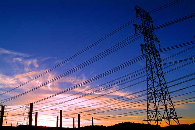
Power Grid

Power grid of the Western States of the USA

$$w(i,j)=\psi(dd \ cdot {i – 1, if k(j)=0k(i), otherwise, 1, 0)$$

The power grid generator also uses the affinity generator, but in a more binary fashion: the weight is always 1 if there is affinity and null if there is not. All the complexity of the generator is captured by the decision on the number of affinity groups. The following things can be noted about the expression that determines the number of groups:

• Overall, the probability of affinity decreases exponentially with distance.
• The node with the sequential identifier 1 overrides the previous rule if the target has no connections, by making the exponent null. This configures a central hub for newcomers to connect to.
• An origin with no connections overrides the previous rule if the target is already connected, also by making the exponent null.

This configures a branching growth behaviour, where new vertices either connect to a central hub or some already connected vertex, but connections between already connected or distant vertices are discouraged. The tree-like structure that originates from this matches our intuitions about the growth of a power grid. The affinity operator, by implicitly using sequence identifiers, might abstract at a high level the underlying spatial constraints.